Hello folks, this is my first blog and starting from here i will put up my knowledge and thoughts on Data Science in the form of this blog's or article's. As i am novice writer /blogger, there will be a chance of mistakes, so please leave a feedback that will help me in future

Let's Start!

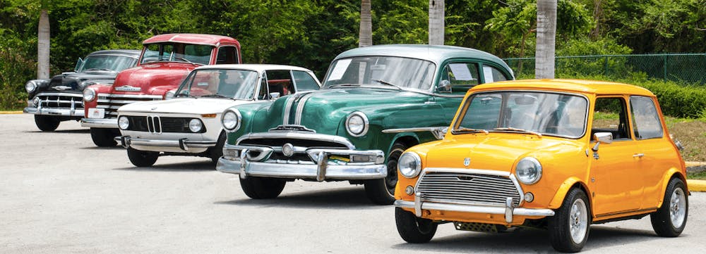
This blog gives you an idea to build a car price prediction system to predict the price of used cars. Through this blog you can also learn several data cleaning and visualizaton techniques used to extract the information from the given data. I ensure you that at the end of this blog you have a confidence to build your model.

You can reach all Python scripts relative to this on my GitHub page .

Need of Car Price prediction System?

The prices of new cars in the industry is fixed by the manufacturer. So, customers buying a new car can be assured of the money they invest to be worthy. But due to the increased price of new cars and the incapability of customers to buy new cars due to the lack of funds, used cars sales are on a global increase.There is a need for a used car price prediction system to effectively determine the worthiness of the car using a variety of features. Also there are many well established firms which offers used vehicles to their customers in affordable price range, they also use machine learning techniques to determine the price of a vehicle to sold. A system to be able to predict used cars market value can help both buyers and sellers.

Content

Topics I covered in this article/project are :

• Justifications during data cleaning(Identifying null values, filling missing values and removing outliers)
• Exploratory Data Analysis (EDA)
• Performing machine learning models: Random Forest, Linear Regression
• Comparison of the performance of the models
• Feature Selection using p-value
• Reporting the findings of the study in notebook's final result

Data

You can get the data used for this project from here Take a quick look to the structure of data table we used.

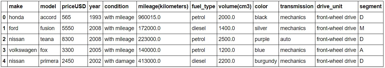
In this dataset our target column is priceUSD and the rest are used as a feature to predict target value.

1. make : Makers or Manufacturer of the car. In simple words car's brand.
2. model : car belongs to which model of specific brand.
3. priceUSD (target) : True market value of car's on which the model trained to predict unknown prices of car's by using rest of the features.
4. year : manufacturing year(1938-2019).
5. condition : current condition of car(with mileage, damage, use for parts) .
6. mileage(kilometers) : how much car travelled till now in km.
7. fuel_type : type of the fuel, in our dataset there is only two options(petrol and diesel) but there are also car's available with CNG.
8. volume(cm3) : Space in car
9. color : color of the car
10. transmission : tell us about the car is automatic or mechanic.
11. drive_unit : defines which drive unit car belongs to.
12. segment : defines segment type of car (for more info, google).

Data Cleaning

Data cleaning is the process of fixing or removing incorrect, corrupted, incorrectly formatted, duplicate, or incomplete data within a dataset. Before cleaning the data we have to understand the terms and information about the data on the basis of which we will proceed for data cleaning.

Easiest and Simplest way to start observing any data is by using panda's describe function which reveals a lot about the dataset. Let's see what happen in our case.

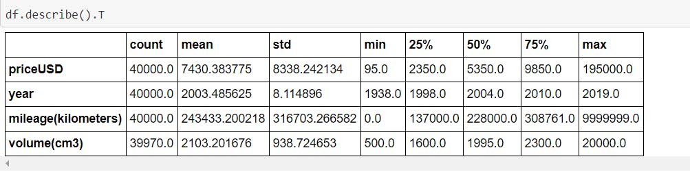
What it reveals ?

• Dataset includes the car from 1938 to 2019 (contain oldest and newest both). 75% of the car's are manufactured after 1998, means not so old cars are there.
• Minimum kilometer travelled by the cars in the dataset is 0, practically which may be not possible because most of the used car are sold after being travelled some distance.(we can see it later while removing outlier)
• Minimum Price of Car is 95 USD and maximum price is 195000 USD and More than 75% of cars are below than 1000 USD. Here most expensive cars seems to be outlier.

As a next step, check missing values for each feature.

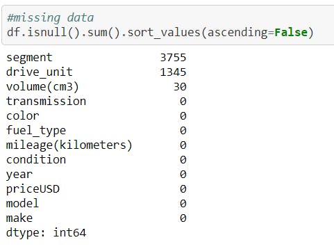Next, now missing values were dropped or filled with appropriate values by an appropriate method. In my case i drop the rows with missing values but you can do experiments by filling them with the mean or median.

After dealing with missing values remove all the duplicate rows from the dataset by using below command.

df = df[~df.duplicated()]

At last, there are zero null values with no duplicates.

Outliers: InterQuartile Range (IQR) method is used to remove the outliers from the data.

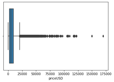
• From figure 1, the prices above 20000 USD(approx.) are the outliers.
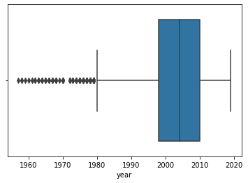
• From figure 2, it is impossible to conclude something so IQR is calculated to find outliers.
• From figure 3, the year below 1980 are the outliers.

df = df[~((df < (Q1-1.5 * IQR)) |(df > (Q3 + 1.5 * IQR))).any(axis=1)]

Exploratory Data Analysis(EDA)

EDA helps in better data understanding by visualizing, summarizing and interpreting the information that is hidden in data. Let's come and explore the data.

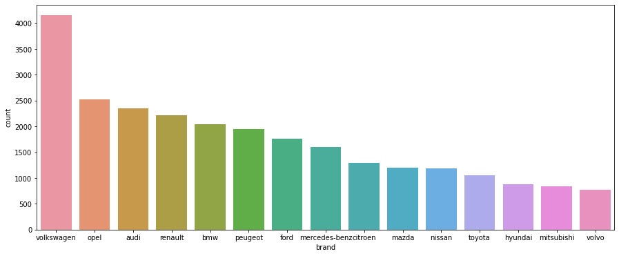By looking at the figure, it can be observed that Volkswagen is the most common brand followed by opel, audi and others in the given dataset.

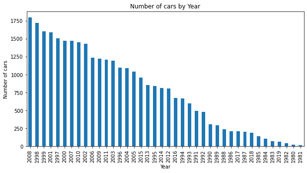
As Dataset contain car's from oldest to newest model but most of the car is from 2008.

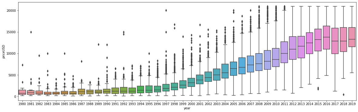Year is an important feature in used car market, as you go from old to new car the price of the car increases, their is a clear increasing tendency. Year of the car impacts on the price of the car.

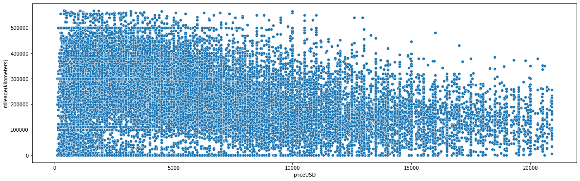
When buying a used car, people pay serious attention to the distance car travelled. We can see mileage has a great impact on the price of a car. Overall Less expensive cars has more mileage as compare to highly expensive cars.

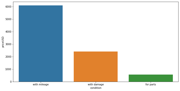This graph indicates that condition is one of the most important feature for price prediction. Damaged cars have less price than one with in good condition whereas cars which can be used for parts after buying is of lowest price.

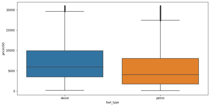
As normal all know diesel car is more expensive as compare to petrol car.

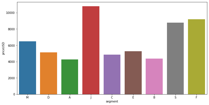
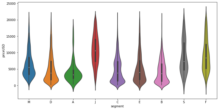
After seeing above two graphs, its clear that segment-J car's price range is highest followed by segment-S car's. Segment-J,S,F cars in the dataset is nearly of all prices or you can say normally distributed whereas others segments cars price are concentrated between some range.

Correlation : With the help of correlation we can easily check which feature strongly connected or in other terms it tells how strongly one feature is related to other. We can check the correlation between variables with the help of Heatmap.

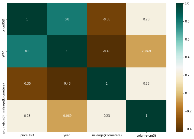
In the above heat map we know that the price feature depends mainly on the year and the mileage as positive and negative correlation respectively.

We saw Nearly all trends and dependencies in above visualization, now let's delete all useless features, I remove two column make and model as it contains only car brands and its models name which will not add much value in prediction.

df.drop(["make"],axis=1,inplace=True)
df.drop(["model"],axis=1,inplace=True)

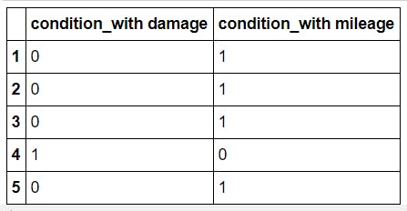
Preprocessing - After deleting this two columns we left with only six categorical column which are transformed in the form of 0 and 1 using get_dummies() function.

Let's see an example by taking a feature, condition.

condition = df[['condition']]
condition = pd.get_dummies(condition,drop_first=True)
condition.head()

Similarly we do this for all the other categorical features as well.

ML Models

Train-test-split : First we are splitting the data to train and test the model. 80% of instances used to fit the models and remains of instances (20%) will be used to compute the accuracy scores of models to avoid overfitting.

from sklearn.model_selection import train_test_split
X_train, X_test, y_train, y_test = train_test_split(X, y, test_size =0.2,random_state=42)

The dataset is supervised, so the algorithm applied are in a given order:

1. Linear Regression
2. Extra Trees Regressor
3. Random Forest Regressor

1) Linear Regression :

In statistics, linear regression is a linear approach to modelling the relationship between a scalar response (or dependent variable) and one or more explanatory variables (or independent variables).

Error table we get after applying Linear regression is :

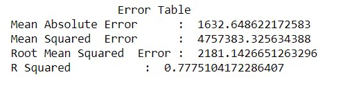
Didn't get a good score, let's try something more better.

So, now I am using Extra Trees Regressor and Random Forest Regressor (obviously for better accuracy)

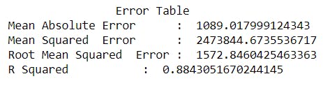
2) Extra Trees Regressor :

This class implements a meta estimator that fits a number of randomized decision trees (a.k.a. extra-trees) on various sub-samples of the dataset and uses averaging to improve the predictive accuracy and control over-fitting.

Error table we get after applying Extra Trees Regressor is :

3) Random Forest Regressor :

Similar to Extra Trees Regressor only difference is the method of choosing the split point for decision trees. Unlike Extra Trees algorithm, which select a split point randomly, Random forest algorithm uses a greedy algorithm to select an optimal split point.

Error table we get after applying Random Forest Regressor is

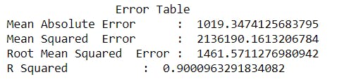
Now after using Random forest we got a good score.

Feature Selection

Accuracy of the model can be increased with the help of feature selection methods. Feature Selection is the process where you automatically or manually select those features which contribute most to your prediction variable or output in which you are interested in. As there are many methods to select features, some of them are feature importance, correlation(more info)

In our case we use p-value for feature selection, so in Regression very frequently used techniques for feature selection are as following:

• Stepwise Regression
• Forward Selection
• Backward Elimination

I will use Backward elimination in this case. In backward elimination in the first step we include all predictors and in subsequent steps, keep on removing the one which has the highest p-value (>.05 the threshold limit). after a few iterations, it will produce the final set of features which are enough significant to predict the outcome with the desired accuracy.

code for checking the p value of each feature with different subsets

X_opt = X.values
regressor_OLS = sm.OLS(endog = y.values, exog = X_opt).fit()
regressor_OLS.summary()

But after taking the subset of features our accuracy does not change a little bit thus we will keep all the previous columns.

You may use Hyperparameter tuning for better result. If this blog is helpful for you then please give a star to the repo on Github .

Thanks for reading, Deepdive into AI !